This section introduces some projects I have done during my master's study

Content
1. Filed work study: Greenhouse gases, Biogeochemical, Sphagnum
2. Climate change and its impacts: Using LPJ-GUESS
3. Extreme event study
4. Climate model study
5. Impacts of climate change on agriculture in Ukraine (literature review)
6. Ecosystem modelling: Biome Modelling
7. Ecosystem modelling: Sensitivity analysis
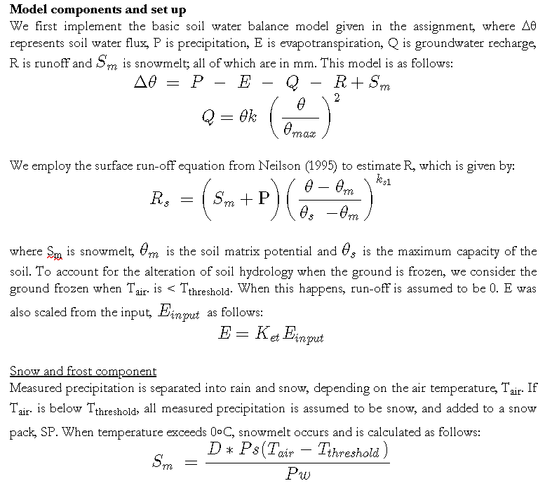
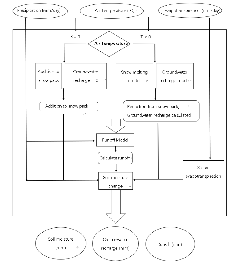
8. Ecosystem modelling: hydrology model
9. Remote sensing: Lunds Kummon project
10. Remote sensing: Timeseries (Using TIMESAT)
11. Programming in GIS and remote sensing: Application project (Using Python)
12. Global ecosystem dynamic: Cropland management (Using Matlab)


Course works and projects: Greenhouse gases and biogeochemical cycles, NGEN14, Lund University


The effect of abiotic factors on the exchange of greenhouse gases in red and green Sphagnum mosses on the Fäjemyr peat bog in Skåne, Sweden (Field work of biogeochemical course)

Intro:In this field work study, the chamber method is used to measure and compare methane and CO2 fluxes of two varieties of Sphagnum moss (red and green one) in Fäjemyr in southern Sweden. Our results do not agree with many previous studies that cite water table depth as the main driver of methane concentration in Sphagnum; it is instead found that the processes of methanogenesis, methane oxidation and photosynthesis are too complex to be attributed to just one abiotic factor.

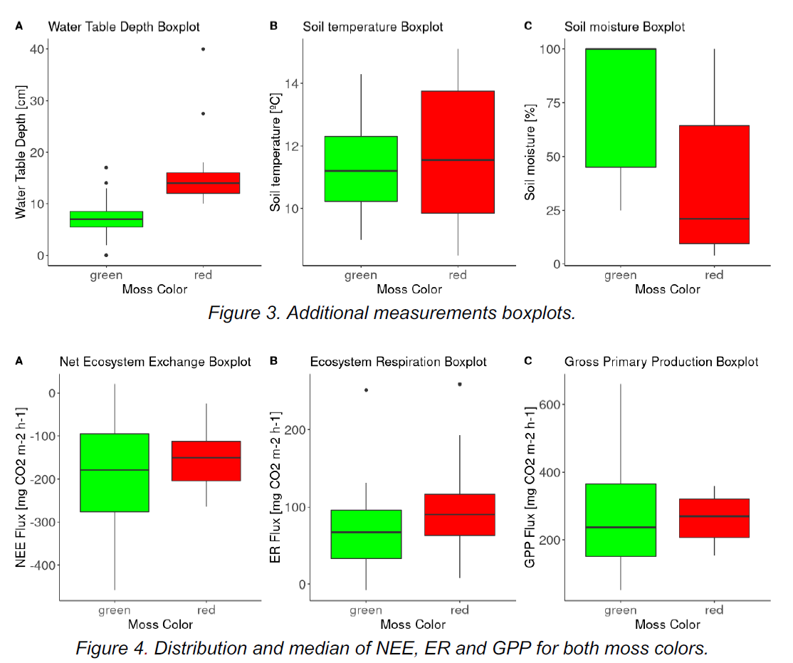
Some insights: Below (noted Figure 3 and 4) depicts how abiotic factors vary between the moss patches. The box plot of NEE (Figure 4.A) shows a greater interquartile range in the green moss, a median of -151 mgCO2 m-2 h-1 for the red and a slightly greater NEE (more negative) for the green (-179 mgCO2 m-2 h-1). For both ER and GPP (Figures 4.B and 4.C) the interquartile range is higher among the green plots, but the median is greater in the red.
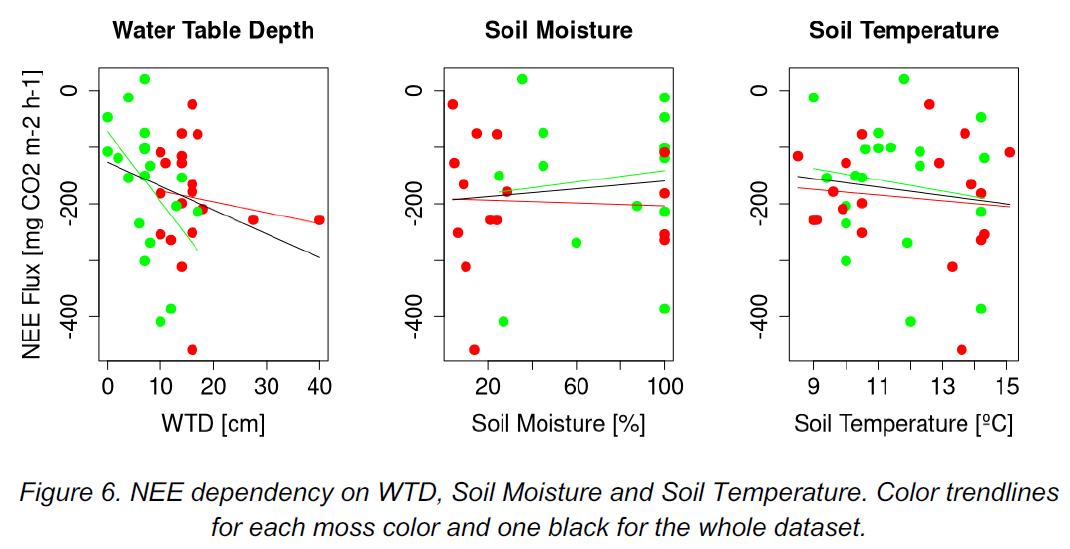
Both colors of Sphagnum show a weak to medium correlation between NEE and soil moisture (noted Figure 6), with a R2 of 23% for the red patches and 41% for the green. It is apparent that the green moss was much wetter than the red (with the exception of 100% soil moisture in the red moss after a high amount of rainfall), which confirms the Wilcoxon result. Neither temperature nor water table depth show significant correlation with NEE. For all green samples with a NEE ~ -400 mg CO2 m-2 h-1, very sunny conditions were noted.
Group 1 in module Greenhouse gases and biogeochemical cycles, NGEN14
Zhicong Xie, Maja Holm, Emily Register, Salvador Hernández, 2021
Course works and projects: Climate change and its impactss on environment, NGEN01, Lund University


Using LPJ-GUESS vegetation response to climate change for 100 years in 3 different sites (Ecosystem modelling work of climate change course)

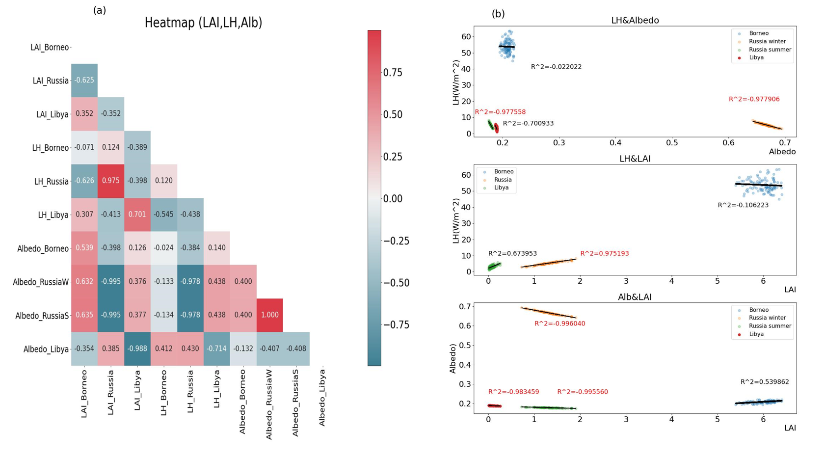
Intro: A vegetation dynamics-based model, LPJ-GUESS was used in this exercise to simulate the vegetation response to climate change for 100 years in 3 different sites (Northern Russia, Borneo, and Libya). Model outputs including leaf area index (LAI) and evapotranspiration were used to calculate albedo and latent heat flux (LH) to analyse the response of vegetation and identify feedbacks in the terrestrial system due to climate changes.
Conclusion: Our simulations show that the response of vegetation due to climate change differs with region. For extremely cold regions like Russia, we clearly see that temperature is the main driver in catalysing vegetation changes, whilst in tropical areas like Borneo, it is difficult to discern a single main factor since different vegetation types respond differently to changes in climate parameters. We also identified a positive feedback loop involving albedo and LH, as well as LAI and LH.
Some figures:

Group of module Climate change and its impacts on environment, NGEN01
Zhicong Xie, Jana Lim, 2021

Extreme rainfall: future trends and health implications

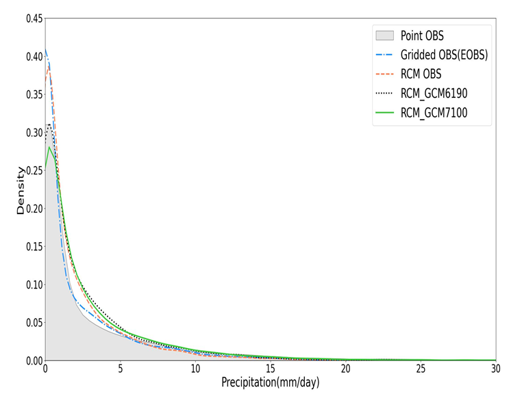
Intro: This report compares precipitation and wet spell outputs from models to observed point and gridded data in Bredeney, Essen in Germany between 1961 to 1990. It also analyses projections on precipitation in future for the years 2070 to 2100. We hypothesise that extreme precipitation events have increased in frequency and magnitude. In turn, this will increase the risk of flooding and hence, increase risks to human health. This study examines the effect that extreme precipitation has on floods and how these affect human health.
Figures:

Group of module Climate change and its impacts on environment, NGEN01
Zhicong Xie, Jana Lim, Maja Källehult, 2021

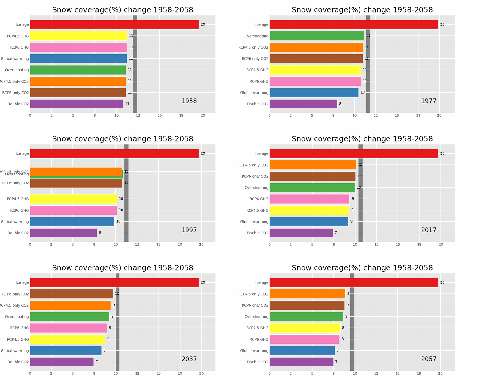
Climate modelling exercise

Snow cover change in different climate scenarios over time:

Group of module Climate change and its impacts on environment, NGEN01
Zhicong Xie, Jesus Mallol Diaz, Vaidehi Singh, 2021

Project work: What are the impacts of climate change on Ukraine’s agricultural sector and the ramifications on food security? (Literature review)

Intro: Climate change can impact agriculture by affecting crop yields. Decreases in yield and its variability can threaten food security and therefore, the health of the general population. Here, we conduct a literature review to investigate how climate change under RCP 2.6 and RCP 8.5 may affect crop production in Ukraine, a major breadbasket region. We found that both the temperature and precipitation are expected to increase, albeit to varying degrees since there is spatial variability in the country’s natural environment. More extreme weather events are projected to happen as well. This could have ramifications for food security in the nation, as well as its major importers. Although the state has recognised the urgent need to make adjustments to strengthen the sector’s resilience to climate change, present measures that have been in place are still inadequate and nascent. Literature on Ukraine’s agricultural sector and its vulnerabilities to climate change are also scarce. Future scientific research is needed to address this knowledge gap to strengthen the resilience of the country’s agricultural sector and food security.
Conclusion: This paper has examined precipitation and temperature projections for Ukraine under RCP 2.6 and 8.5. Increases in the extreme and mean temperature and precipitation are likely to adversely affect the agricultural sector. As a major breadbasket, this may have far-reaching consequences on food security beyond the nation’s geographical borders. Whilst the nation has acknowledged the need to mitigate the sector’s risk to climate change, it is unclear what course of action will be taken. Ultimately, the impacts of climate change on agriculture are highly complex since it is an interplay between processes that may be environmental, economic and technological. Hence, more research has to be done to better understand the country’s agricultural sector. This would provide a strong foundation for measures which could be adopted to strengthen the sector’s resilience to climate change to ensure food security. Thorough scientific research on the country’s agricultural sector would be a crucial first step.

Group of module Climate change and its impacts on environment, NGEN01
Zhicong Xie, Jana Lim, 2022

Course works and projects: Ecosystem Modelling, NGEN02, Lund University


Biome Modelling

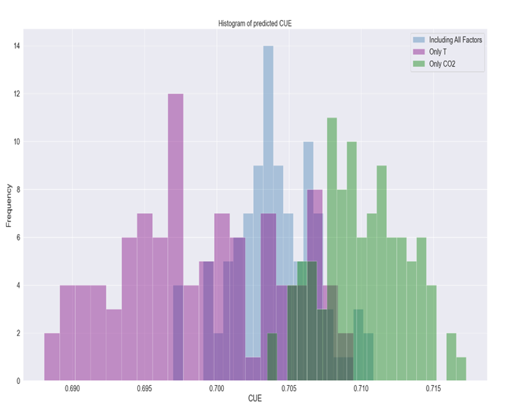
Intro: A vegetation dynamics-based model, LPJ-GUESS was used in this exercise to simulate the vegetation response to climate change for 100 years in northern Russia. Model outputs including leaf area index (LAI), NPP and GPP were used to calculate albedo (Both summer and winter) as well as Carbon Use Efficiency to analyse the response and processes under ecosystem and identify the main drivers in the terrestrial system due to climate change.
Discussion (excerpts): Generally, both the albedo and carbon use efficiency decrease due to climate change. However, different factors have different impacts. In addition, the total LAI increase sightly with future changes. emperature is the most influential factor in albedo changes. The albedo decreases around 0.03, which is much higher than the other 2 factors. This makes sense because first of all, in winter, the temperature can influence the snow melting, and snow cover area and thickness are critical to reflectivity. In summer, higher temperature means the vegetation growth period is prolonged, thus promoting the plant and microbes’ growth. This can increase LAI, thereafter increase canopy shading and decrease albedo finally. In addition, evapotranspiration will increase and increase the root water uptake and reduce soil wetness. If without allochthonous water and nutrient supply, this imbalance may make this region dry and then damage the ecosystem.
Some figures:

Individual work of Ecosystem Modelling, NGEN02
Zhicong Xie, 2022

Sensitivity analysis

Intro:In this exercise you will use a Monte Carlo approach to assess the sensitivity of LPJ-GUESS to uncertainty in some of its paramete.
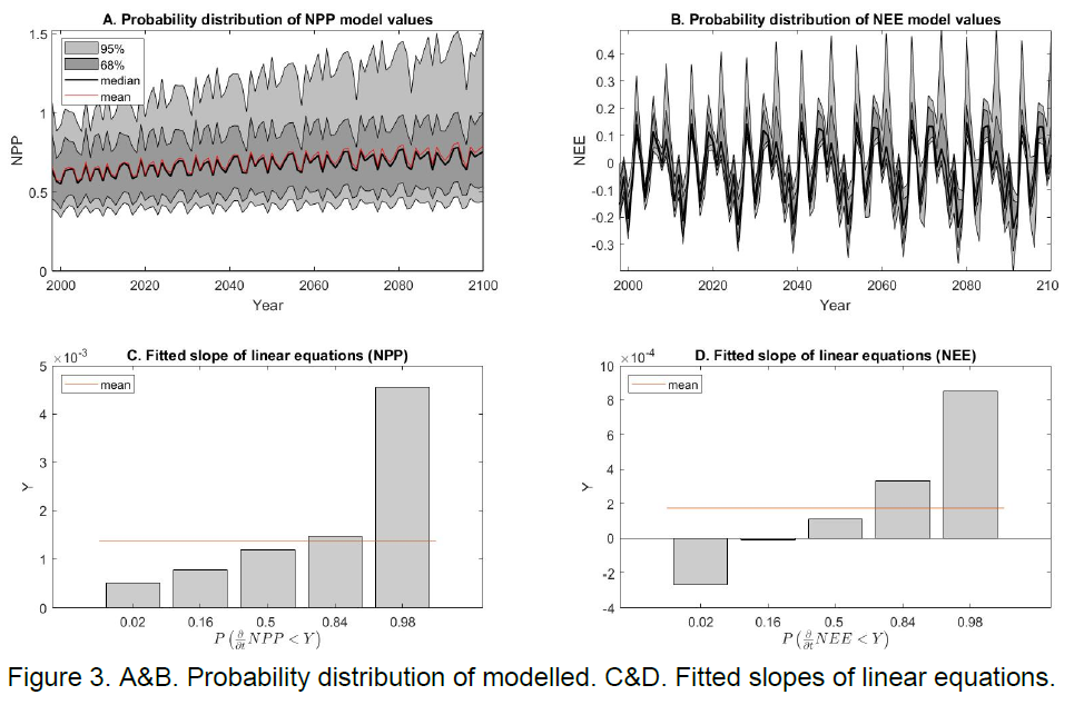
Discussion (excerpts): The timeseries for monthly NEE for Hyytiala, Finland is shown in Figure 1. About half of the observations (n=19) do not fall under the range of uncertainty. This may be due to:
—— A difference in scale - since LPJ-Guess assumes each modelled area to be large (~100km2), hence, the output of the model is generalized over a large area (where there is likely to be spatial variability), as opposed to the observed data which is a point and therefore more much more localized
—— Inherent uncertainty in the ‘correct’ parameters used – both in terms of value and whether or not it should be represented in the model in the first place
—— Inaccuracy in the Euroflux data; it is possible that the measurement tool was faulty, or that it was derived from a model with some errors.
Some figures:

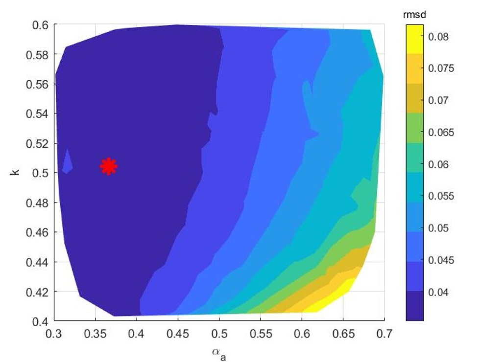
Parameter sensitivity (αa& k):Factor αa is the most significant parameter of NPP Rh and NEE for Finland

In terms of robustness, the model appears to be much better at predicting NPP as compared to NEE. A Mann-Kendall test on both time series confirmed the presence of a trend. Thereafter, linear equations were fitted for values at the 2nd, 16th, 50th, 84th and 98th percentile (Figure 3C and 3D) for both NPP and NEE. These were chosen since they correspond to being 2 and 1 standard deviations away from the mean in both directions under a normal distribution. From Figure 3C, we see that the probability of obtaining a slope < 0.0005 is less than 2% for NPP, and that there’s a 96% probability that a fitted slope lies between 0.0005 and 0.005. This suggests that it is extremely likely that NPP is increasing. However, Figure 3D shows that there is at least a 16% probability of obtaining a slope less than –9.0, but there is a 48% probability of obtaining a slope between 0.001 and 0.009. This shows a higher degree of uncertainty in predicting NEE.

Group of module Ecosystem Modelling, NGEN02
Zhicong Xie, Jana Lim, 2022

Project work: Ecosystem hydrology model

Intro: Here, we constructing a dynamic ecosystem hydrology model of a forest at the stand scale. This model is tested out on a study site, Hyytiala in Finland. We first explain the steps taken to set up the model, calibrate empirical parameters and validate the model in our methodology section. Thereafter, we test both the parameter and climate driver sensitivity, to see how these variables will affect the model outcomes.
Design: Here are some excerpts

Reference:
McGinn, R. A. (2012). Degree-Day Snowmelt Runoff Experiments; Clear Lake Watershed, Riding Mountain National Park. Prairie Perspect. Geogr. Essays, 15, 38-53.
Muskett, R. R. (2012). Remote sensing, model-derived and ground measurements of snow water equivalent and snow density in Alaska.
Neilson, R. P. (1995). A model for predicting continental‐scale vegetation distribution and water balance. Ecological Applications, 5(2), 362-385.
Zhou, G., Cui, M., Wan, J., & Zhang, S. (2021). A Review on Snowmelt Models: Progress and Prospect. Sustainability, 13(20), 11485.

Diagram: More details and discussions are not presented here because it is a complex work.

Group of module Ecosystem Modelling, NGEN02
Zhicong Xie, Jana Lim, 2022

Course works and projects: Remote sensing, NGEN08, Lund University


Lunds kummon project

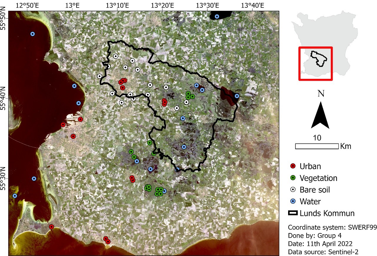
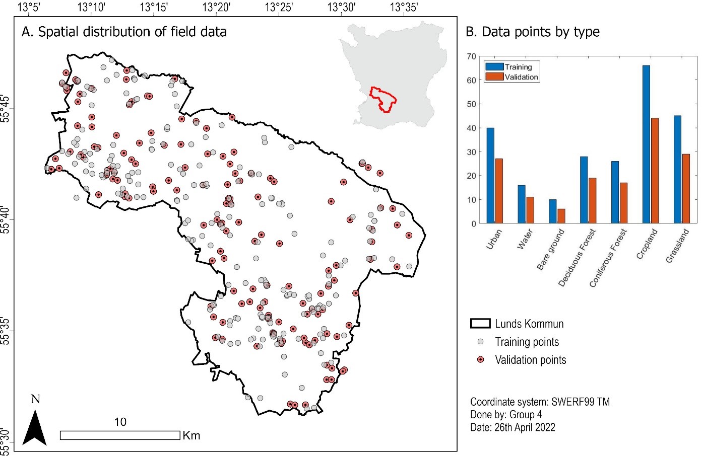
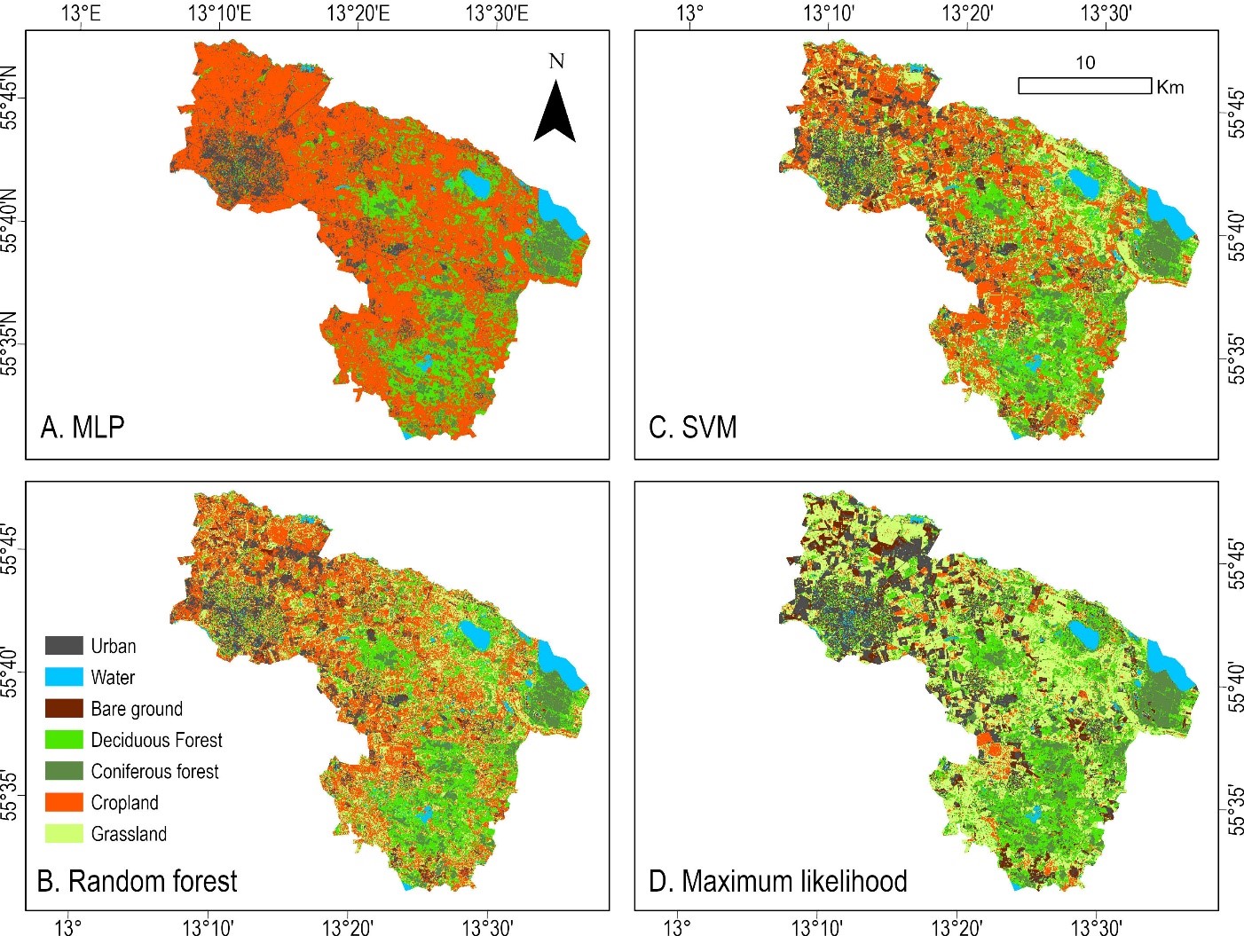
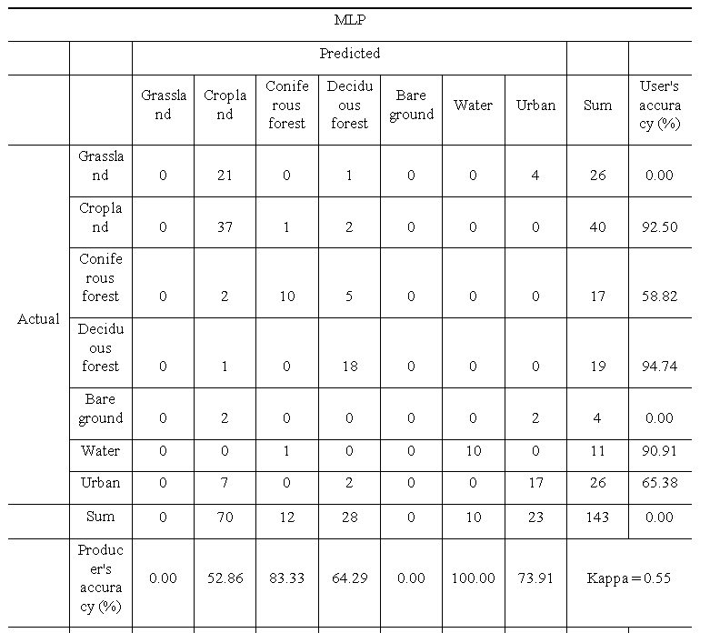
Intro: In this exercise, we sought to measure, compare and account for the differences in the results and accuracy of 9 land cover maps (10m) that were generated over Lunds Kommun, a 44km2 area located within the Skåne municipality of Sweden, using a Sentinel-2 image. A preliminary land cover map was first generated using training points that digitized via manual inspection of the Sentinel-2 image. Thereafter, 8 land cover maps were generated using field data collected on a single trip in April 2022. These land cover maps were generated using various machine learning methods – maximum likelihood (ML), multilayer perceptron (MLP), random forest (RF) and support vector machine (SVM) – and band combinations – true colour, and false colour composites. The accuracy of these maps was measured using the Kappa Index.
Conclusion:Our findings indicate that various machine learning algorithms have varying levels of accuracy when generating land cover maps. There is also differences in results from using a false and true colour composite to generate land cover maps. Except for the MLP algorithm, we see that results from the true colour composite returns a better Kappa coefficient compared to the false composite. The SVM also returns the best Kappa coefficient among the algorithms. In terms of Kappa value, it is suggested that land cover maps generated from field data may be slightly more accurate than those generated solely by training points based on the satellite imagery, although this would require a fairer comparison with standardization of categories and the time in which training points were generated.

Some figures:

Distribution of sampling points for the pre-classification land cover map.

A. Field data points. B. Number of data points per class.

Land cover maps generated using the false colour composite.

Confusion matrix for machine learning (False colour composites)

Group of Module Remote sensing, NGEN08
Zhicong Xie, Jana Lim, Jesus Mallol Diaz, Leo Petersson, 2022

Timeseries exercise

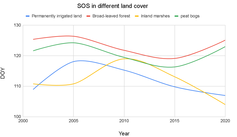
Intro:Phenology refers to the study of how biological organisms respond to changing environmental factors (normally periodic changes), such as precipitation, temperature and water content and their interrelationship. Also, seasonal and interannual variations in climate are important indicators in climate change studies. The study of phenology can help us to evaluate the overall effect of environmental factors on the impact of plants and animals. The plant phenology index is a new vegetation index used for monitoring plant phenology and developed for time-series analysis based on the physical principle of radiative transfer (Jin & Eklundh, 2014). In this exercise, we investigated the phenology variables (EOS, SOS, LOS) in different land cover types and their controlling factors by using a time-series analysis software (TIMESAT).
Discussion (excerpts): We basically divided our study area into 4 parts based on land cover types. As shown in Figure below, the start of the season (SOS) ranges from around day 110 to 130 (approximately April to May) over the 20 years (2000-2020) with some variations and varies in different land cover types. Compared to the other 3 land covers, the SOS in Broad-leaved forests is the latest every year (DOY: 120-135), followed by the peat bog, which is a little earlier entered the growing season. The season seems to start earlier in inland marshes and irrigated land (DOY: ~110). The SOS difference between Broad-leaved forests and inland marshes is around 10 days and up to 20 days, with the exception of the year 2010, which is a huge difference.
In terms of the end of season (EOS), it is showing a totally different pattern than SOS (Figure 3.). The end of the seasonal period is the latest in inland marshes (range from day 230 to 260, August and September). However, the growing season of the other 3 types ends in the same period (around day 220 to 225). The EOS difference between inland marshes and the others is about 10 days, but up to 50 days in 2015 (eg. Permanently irrigated vs. Inland marshes)
Some figures:

Start of season (SOS) in 4 land cover types.

End of season (EOS) in 4 land cover types.

Group of Module Remote sensing, NGEN08
Zhicong Xie, Leo Petersson, Wenjing Liu, 2022

Course projects: Python programming in GIS and Remote sensing, NGEN20, Lund University


Course project

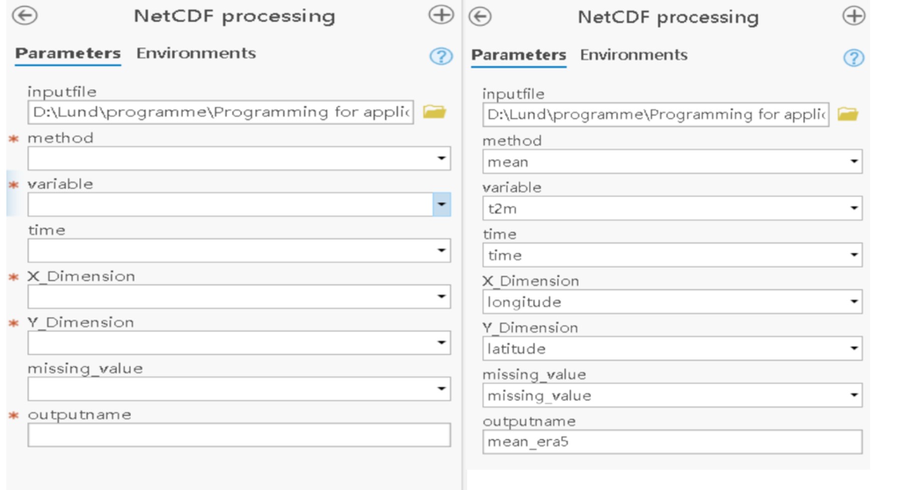
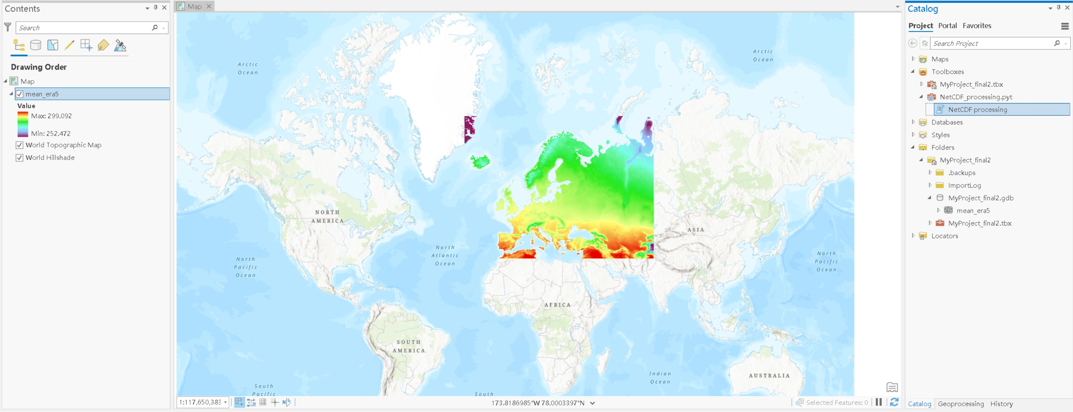
Intro: In this project, I am going to seek a way to create a Python toolbox used in ArcGIS Pro in which users can quickly and conveniently process nc files. Hence, those who do not want to (or do not know how to) process nc files can easily implement it in ArcGIS pro. Three variable indices are involved in this toolbox: Mean, Trend, and Amplitude. Given an nc input file, users are guided to enter a few related parameters (Some are required and some are optional). The results (raster format) will be displayed in the current map with defined symbology and stored in working space properly, general information about the data you input and the method selected can be traced in the message window after implementation.

Conclusion:This Python toolbox provides mean, trend, and amplitude calculations and output in the format of raster when proper format nc file data is given. It allows users to obtain general but valuable information from geospatial data in a short time. This saves time and avoids processing messed-up data. With output data, users can do further geospatial analysis combine with their dataset.

Some figures:

Toolbox interface.

Results shown on ArcGIS pro

Zhicong Xie, 10-2022

Course works: Global ecosystem dynamic, NGEN17, Lund University


Course exercise: Mitigation in agriculture

Intro: Climate change has great influence on agriculture by affecting the emissions of crops as well as crop yields. Decreases in yield and its variability can threaten food security, and therefore human beings. Greenhouse gases emitted from agriculture (mainly CH4, N2O) is an important contributor when considering global warming. There is a lot of potential for conducting mitigation in agriculture sector. In this exercise, we estimated the N2O emissions and yields of different cropland management measures by following the works (Olin et al., 2015) and data from LPJ-GUESS simulations.

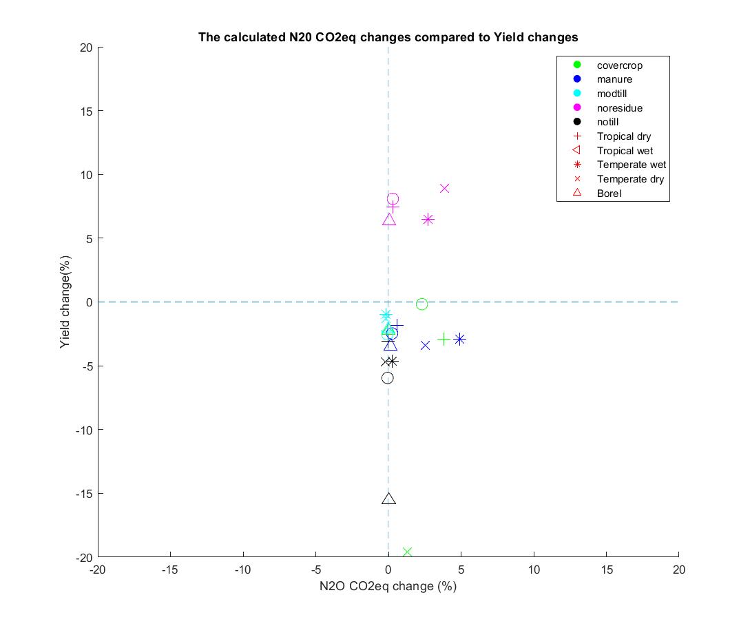
Results:From figure we can know the treatment ‘noresidue’ has positive effect on crop yields (increased 5 to 10 percent, varies in different regions). The boreal area under ‘noresidue’ treatment can represent a win-win situation (Olin et al., 2015) as it can boost yields without increasing N2O emissions. By contrast, the temperate dry region under ‘covercrop’ treatment may not represent an ideal situation since it has great effect on yields reduction, the same happens on boreal under ‘notill’ management. The ‘modtill’ and ‘notill’ measures have sightly mitigation effect on N2O emission (up to 0.20%), with around 5% yields decreases. Therefore, they are also a good choices when we want to balance yields and GHG emission at the same time, and in this regard, sacrifice some of productions to reduce emissions sometime could work.

Some figures:

The simulated relative response (%) of N2O CO2-equivalents to management options compared to the standard set-up in different climatic regions

Zhicong Xie, 11-2022